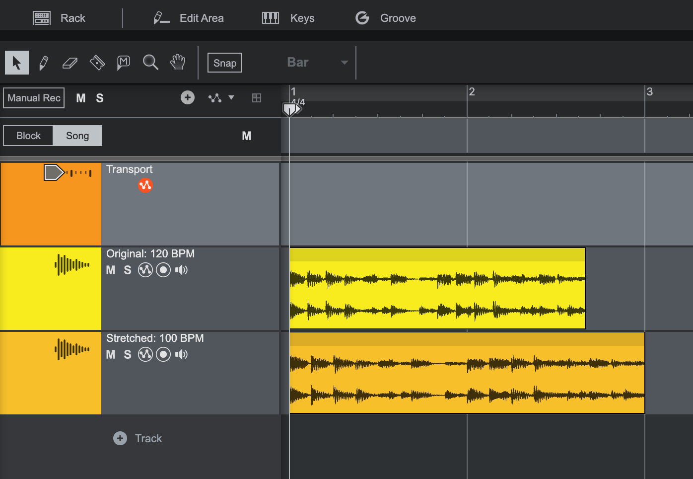
Time stretching algorithms let us change the duration of a recording without changing its pitch. Slow a vocal down, fit a drum loop into a different tempo, or extend a note, and the software has to rebuild the audio so its musical timing changes while its frequencies stay put.
In my article on the Auto-Tune algorithm, I explained how pitch correction changes notes while preserving the duration of a performance. Time stretching tackles the complementary problem. In fact, we can combine time stretching with a change in playback rate to produce a pitch shift.
As a computer engineer who also produces music, I’m interested in what happens underneath those stretch and warp controls. Why can one setting preserve a vocal but turn a snare into mush? The answer comes down to how the algorithm reconstructs the waveform.
Why Changing Playback Speed Also Changes Pitch
A digital recording contains amplitude samples at a particular sample rate. At 48 kHz, one second contains 48,000 samples per channel.
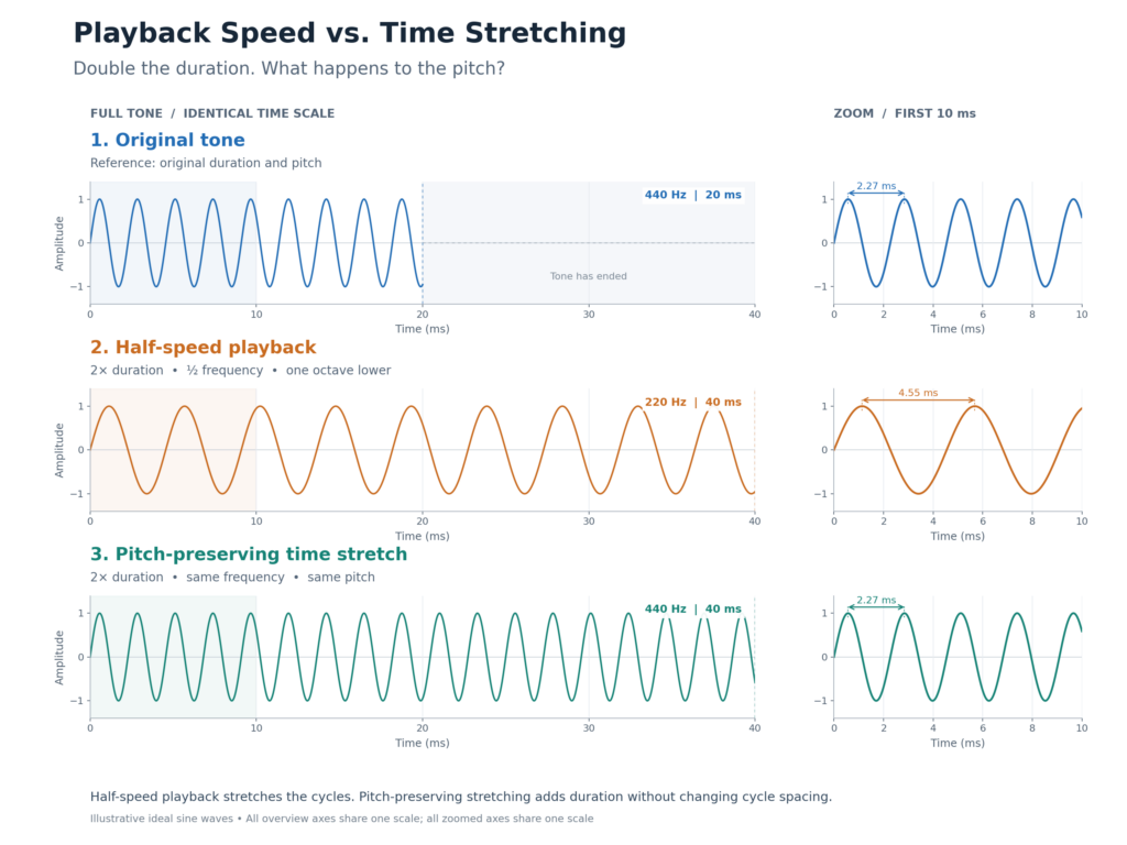
Play those samples twice as quickly and the recording ends in half the time. However, every waveform cycle also passes twice as quickly, so every frequency doubles. A 440 Hz note becomes 880 Hz: one octave higher.
Play at half speed and the opposite happens. The recording lasts twice as long, and the note drops an octave. This is the familiar relationship between speed and pitch on tape machines and turntables.
Time stretching has to separate those two effects. A singer’s phrase might take six seconds instead of five, but an A4 should still oscillate at roughly 440 Hz during a sustained note.
Simply interpolating extra samples between the originals won’t solve that problem if we use them to extend playback at the same sample rate. That stretches the cycles too, lowering the pitch.
Stretch Ratio vs. Playback Speed
For this article, the stretch ratio means:
stretch ratio = output duration / input duration
A ratio of 1.2 makes the recording 20% longer. A ratio of 0.8 makes it 20% shorter.
For a constant-tempo loop that must keep the same number of beats:
stretch ratio = original BPM / target BPM
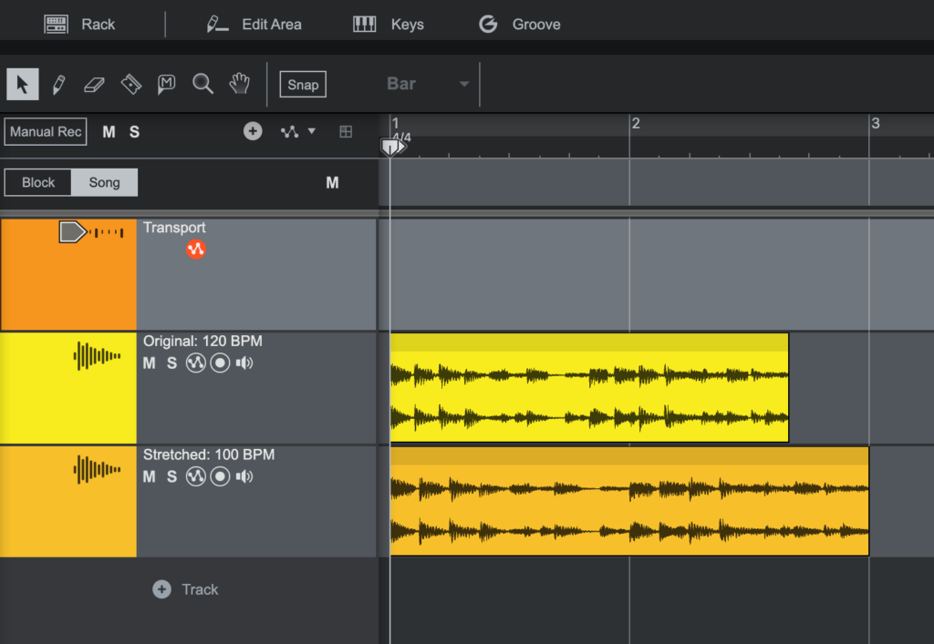
Take a four-bar loop in 4/4 at 120 BPM. Its 16 beats last eight seconds. To fit those beats into 100 BPM:
120 / 100 = 1.2
The new duration becomes 9.6 seconds. The tempo falls by about 16.7%, even though the duration increases by 20%. Those percentages describe reciprocal quantities.
Check your software’s definition: some tools request a speed multiplier instead. In that convention, this example uses 100 / 120, or approximately 0.8333.
How Time Stretching Algorithms Reassemble Audio
Many methods analyze overlapping sections of the input and reconstruct them on a different timeline. The important distinction is between the timing inside a section and the position of that section in the overall recording.
Overlap-Add: The Starting Point
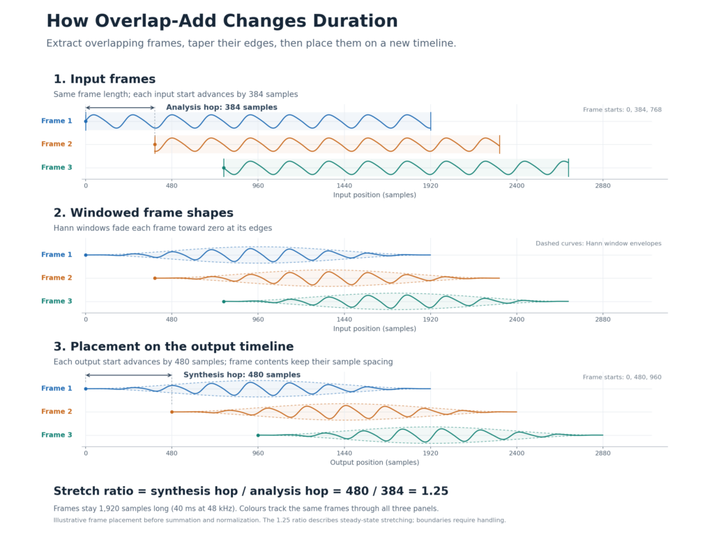
Overlap-add, or OLA, divides audio into short frames. A window function fades each frame toward its edges, and the processor adds overlapping frames together to form the output.
Two distances control the timeline:
- Analysis hop: the distance between successive frame positions in the input.
- Synthesis hop: the distance between successive frame positions in the output.
For a fixed-hop arrangement, the approximate stretch ratio is:
stretch ratio = synthesis hop / analysis hop
For example, take 40 ms frames from a 48 kHz recording. Each frame contains 1,920 samples. Advance through the input by 384 samples, but place successive frames 480 samples apart in the output.
480 / 384 = 1.25
Ignoring boundary handling, we have a recording about 25% longer. Frames still overlap substantially, and their internal sample spacing stays unchanged.
The processor also needs suitable windows and overlap normalization to avoid unwanted changes in volume. The audiotsm documentation exposes these frame and hop parameters directly.
But overlapping frames don’t necessarily agree. If a waveform peak in one frame meets a trough in the next, they partially cancel. Smooth fades can hide abrupt cuts, but they don’t guarantee coherent waveform cycles. Basic OLA therefore provides a starting point rather than a universal solution.
WSOLA: Finding Waveforms That Match
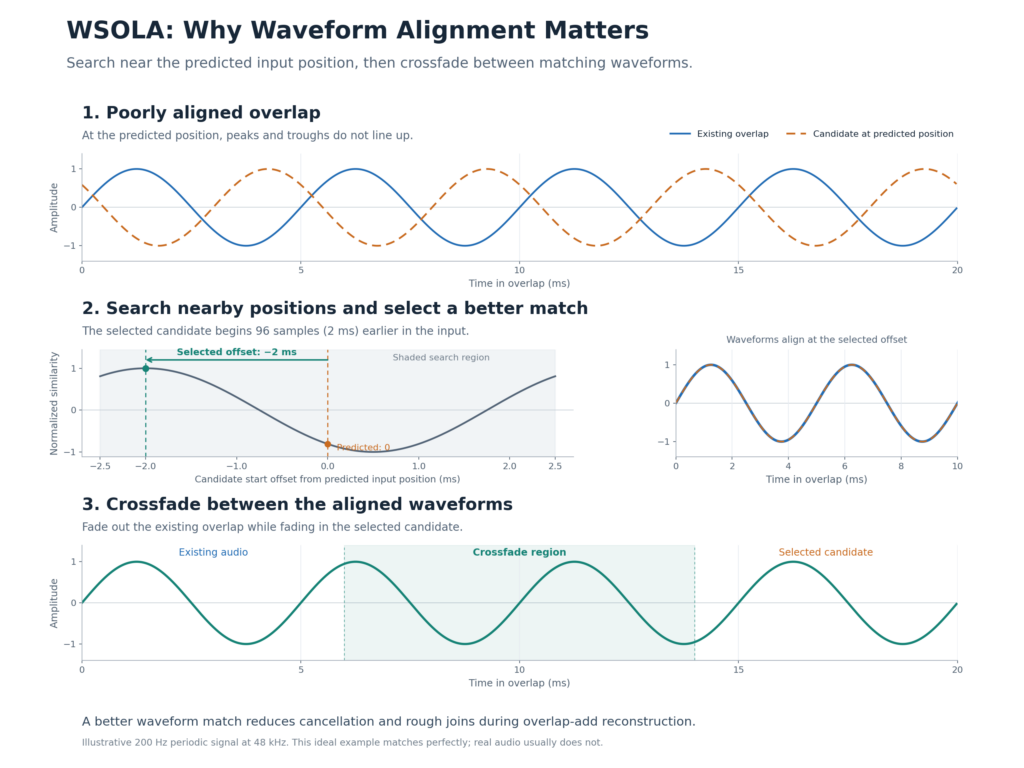
WSOLA stands for Waveform Similarity Overlap-Add. It improves the joins by allowing a small adjustment to each input frame’s position.
Instead of taking the next frame exactly where the stretch ratio predicts, the processor searches nearby positions. It compares candidate overlap regions with the existing audio and selects a close match, commonly using cross-correlation.
Imagine extending a sustained bass note. Shifting a candidate frame slightly can line up its repeating cycles with the previous frame. The processor then crossfades between waveforms that reinforce each other instead of fighting.
This local search doesn’t replace the overall timing target. It gives the processor some freedom around that target to make a cleaner join. MathWorks documents this alignment search in its WSOLA implementation.
How This Relates to PSOLA
Pitch-Synchronous Overlap-Add, or PSOLA, uses pitch periods as its reference. For time stretching, it can repeat or omit pitch-centered grains while keeping the output pitch-mark spacing appropriate for the original note.
That differs from changing the spacing to shift pitch, as discussed in the Auto-Tune article. Both operations rearrange small waveform sections, but they change different relationships between the input and output timelines.
Pitch-synchronous processing suits a clear single voice more naturally than a full mix. A chord contains several simultaneous periods, so one set of pitch marks cannot describe every note.
The Phase Vocoder: Stretching in the Frequency Domain
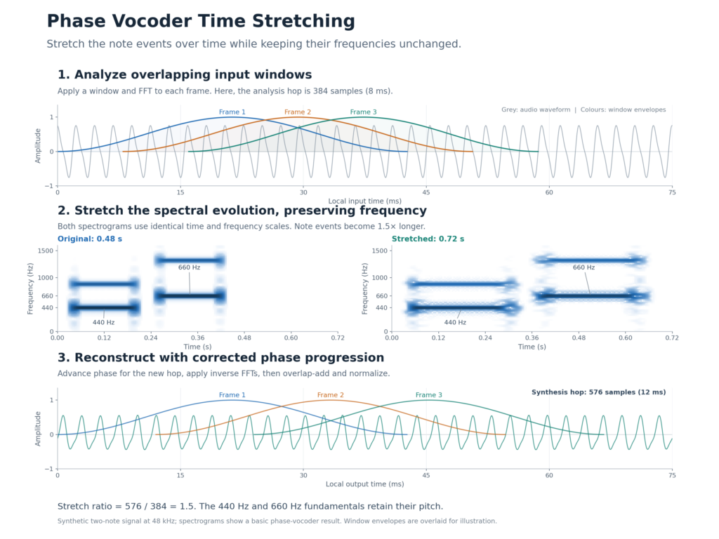
A phase vocoder approaches the problem through frequency analysis. It doesn’t need to find one repeating waveform period that describes the whole recording.
Analysis With the STFT
The processor divides the signal into overlapping, windowed frames and applies a Fast Fourier Transform to each. Together, these transforms form the Short-Time Fourier Transform, or STFT.
Each frequency bin contains two useful values:
- Magnitude: how strongly that frequency region contributes.
- Phase: where the component sits within its oscillation cycle.
The processor creates a new sequence of spectra on the output timeline. Conceptually, it stretches the spectrogram along the time axis while retaining its frequency structure. Dan Ellis’s phase vocoder explanation and implementation demonstrate this approach.
However, moving spectral frames without correcting their phases won’t reconstruct the original frequencies reliably. Magnitudes describe only part of the sound.
Why Phase Must Advance Correctly
Suppose we track a steady 440 Hz component. At 48 kHz, an output hop of 480 samples spans 10 milliseconds. During that interval, the component completes 4.4 cycles.
Its phase must advance accordingly, even if the processor moves through the input at a different speed. Otherwise, adjacent reconstructed frames disagree about the oscillator’s position.
In simplified form:
output phase advance = 2 * pi * frequency * synthesis hop / sample rate
The hard part is estimating the frequency accurately. A real sinusoid rarely lands exactly at an FFT bin’s centre. The processor compares phase changes between input frames with the changes expected at the bin frequency, then uses the residual difference to refine its estimate.
Finally, it accumulates output phases, applies inverse FFTs, and overlap-adds the reconstructed frames.
This lets the spectral content progress more slowly or quickly while the underlying oscillations continue at approximately their original frequencies.
Phase Coherence and Window Length
Keeping a bin consistent over time doesn’t automatically preserve its relationship with neighbouring bins. Modern phase vocoders often use phase locking to maintain relationships around spectral peaks, reducing the diffuse or hollow quality of basic implementations.
Window length creates another compromise. At 48 kHz, a 2,048-sample frame spans about 42.7 ms, with FFT bins roughly 23.4 Hz apart. Longer windows provide finer frequency resolution but cover more time, making rapid events harder to localize.
Shorter windows localize attacks better but resolve nearby low-frequency components less clearly. No single window length perfectly describes a deep bass note and a sharp hi-hat at the same time.
Why Time Stretching Algorithms Produce Artifacts
The difficulty is that musical sounds contain different structures. Sustained harmonics benefit from continuity, while a drum attack depends on a brief, precisely timed event.
Smeared Attacks and Repeated Transients
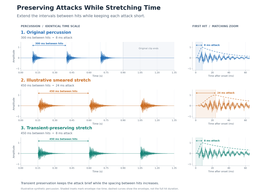
A snare’s initial crack should remain short even when the interval before the next snare grows. Stretch that attack along with everything else and it loses definition.
Time-domain methods can instead repeat or skip an attack as they rearrange frames. What should sound like one hit may become a flam or disappear from the expected position.
Frequency-domain methods can spread transient energy through time. The result may resemble softened percussion or sound leaking ahead of an attack.
Phasey Vocals and Unstable Tone
An exposed voice makes reconstruction errors easy to hear. Poor waveform alignment can introduce cancellation, while disrupted spectral phase relationships can make a vocal sound diffuse or metallic.
Breath, consonants, vibrato, and reverberation also change continuously. Extending them exposes different problems from extending a steady vowel. A successful result on one held note doesn’t prove that a setting will handle the entire phrase.
Stereo Image Changes
Left and right channels contain related timing and phase information. If a processor chooses different frame alignments independently for each channel, it can disturb those relationships.
The SoundTouch documentation specifically warns against treating stereo audio as two unrelated mono streams. Listen for a wandering centre or a change in width, and check mono compatibility when stretching stereo recordings.
How Modern Time Stretching Algorithms Preserve Transients
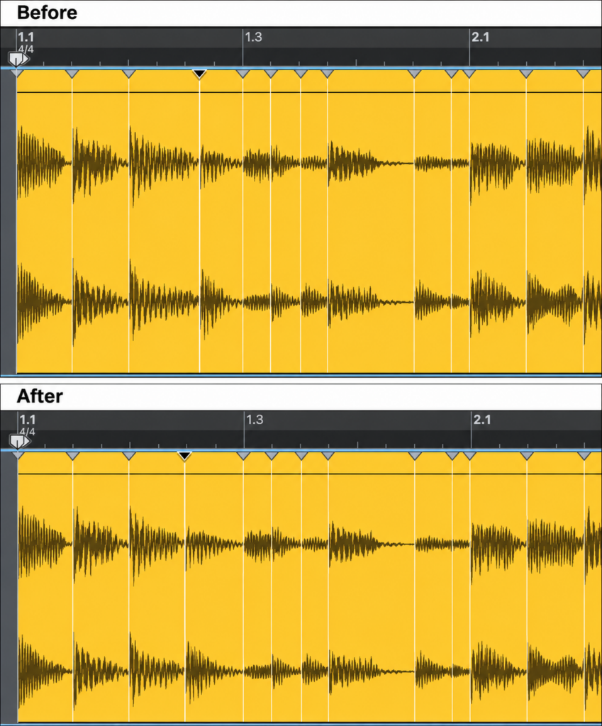
More advanced processors adapt their treatment to the sound. They may detect attacks and preserve those regions near their original duration, then apply more stretching to the sustained material between them.
Some methods reset phase around attacks. Others separate harmonic and percussive components, stretch them using different techniques, then recombine the results.
Driedger and Müller’s review of time-scale modification explains these complementary approaches. Rubber Band’s R2 technical notes describe a concrete implementation using transient phase resets, adaptive stretching, and phase-coherence improvements.
These methods explain why a polished commercial engine can sound substantially better than a basic textbook algorithm. They don’t establish the internal design of every DAW mode: vendors may use proprietary or hybrid techniques.
Choosing Time Stretching Algorithms for Different Sounds
Treat the following as starting points for comparison. The implementation and the amount of stretching matter as much as the algorithm family.
| Source material | Useful starting approach | Listen for |
|---|---|---|
| Dry solo vocal or monophonic instrument | Monophonic, pitch-synchronous, or waveform-aligned processing | Warbling, rough consonants, repeated breaths |
| Drum loop | Transient-preserving or slicing-based processing | Softened attacks, doubled hits, gaps |
| Chords, pads, or sustained polyphonic audio | Phase-coherent spectral processing | Phasiness and unstable sustained notes |
| Full stereo mix | A mode designed for complex musical material | Lost punch and stereo changes |
| Creative textures | Granular or deliberately extreme stretching | Whether the artifacts serve the sound |
For example, Ableton’s Warp Mode documentation distinguishes Beats, Tones, Texture, Re-Pitch, and Complex modes for different material. Re-Pitch deliberately links tempo and pitch; it doesn’t preserve pitch during a tempo change.
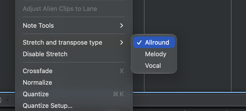
Mode names describe intended use more reliably than they reveal internal engineering. Compare the actual output instead of assuming the most demanding setting will always sound best.
A Practical Listening Test
Use the 120-to-100 BPM example from earlier:
- Choose a correctly trimmed four-bar loop and confirm its original tempo.
- Set the target to 100 BPM with pitch preservation enabled.
- Compare two suitable stretch modes at similar perceived loudness.
- Listen separately to the attacks, sustained notes, and spaces between hits.
- Check the stereo result in mono, then hear it in the arrangement.
If a drum attack suffers, try preserving or isolating it and stretching the following decay instead. If only one syllable needs correction, work locally rather than extending the entire vocal phrase.
Return to the original recording for comparisons. Repeatedly rendering and re-stretching an already processed file can compound reconstruction errors.
Use a lossless working source where possible. My WAV vs FLAC vs ALAC comparison covers those formats, but the important distinction here is simple: a lossless format preserves the samples you give it. It doesn’t undo artifacts that stretching has already introduced.
The Connection Between Time Stretching and Pitch Shifting
We can combine pitch-preserving stretching with a playback-rate change to alter pitch while restoring the original duration.
Start with four seconds of audio. Stretch it to eight seconds without changing pitch, then play that result at twice the rate. The output lasts four seconds again, but every frequency doubles: one octave higher.
More generally, for a desired frequency multiplier p, one approach stretches the duration by p, then applies a playback-rate multiplier of p. The duration changes cancel, leaving the pitch change.
That connection helps explain why pitch shifters and time stretchers share so much signal-processing machinery. Pitch correction adds decisions about which notes to target and how quickly to approach them.
Final Thoughts on Different Time Stretching Algorithms
Time stretching algorithms preserve pitch by rebuilding audio on a new timeline. Waveform-based methods depend on good joins; phase vocoders depend on coherent spectral reconstruction; advanced engines adapt around transients and mixed material.
Understanding those tradeoffs makes stretch controls easier to use. When the result sounds wrong, identify what changed: the attack, the sustained tone, the vocal detail, or the stereo image. Then compare a method designed to preserve that part of the sound.


Leave a Reply